Part II
TACTICS 101: ANTI-SUBMARINE WARFARE (ASW): PART 2 – THE TOOLS OF ASW
In Part 1, we learned the basics of naval oceanography, and in large part, how sound behaves in the subsurface ocean environment.
Now, in Part 2, we move to the tools of anti-submarine warfare (ASW), the sensors, platforms, and weapons. Much of the material contained here is probably “old hat” to seasoned Harpoon players, and certainly generally available to anyone who is willing to take the time and effort to dig up the information.
The purpose of this “Tactics 101” discussion, however, is to provide a workable foundation for those who may be completely new to naval warfare and its concepts. Part 2 tries to touch on many of those concepts.
A. ANTI-SUBMARINE WARFARE (ASW): A VERY SHORT HISTORY
War never changes (there’s my Fallout 3 quote of the day :P), but in the case of anti-submarine warfare (ASW), it has perhaps changed just a little.
The emergence of unrestricted submarine warfare in World War I and the early days of World War II led to grievous (and unanticipated) losses among all major naval powers and their merchant navies, and in turn, threatened both their economic lifelines (the sea lines of communication, or SLOC) and their only means of deploying troops to distant foreign shores.
The danger now posed by submarines to what had been, up to that point, somewhat of a grand surface war, was not particularly welcomed by those on the receiving end. In the words of the First Sea Lord, Admiral Lord Charles Beresford, circa 1900, submarines are “under-handed, under-water, and damned un-English”!
World War II was a watershed event for several major developments in undersea warfare. The Battle of the Atlantic saw the Kriegsmarine’s U-boats pitted against emergent (and increasingly potent) ASW technologies as American and Allied forces herded their convoys to Europe. In the Pacific, US Navy submarines waged their own offensive war against Japanese SLOCs. The development of active sonar or ASDIC, believed to be an acronym for “Allied Submarine Detection Investigation Committee” (but in any event, with Canadian roots. Ahem! ), is a prominent example of emerging ASW technology during WWII.
Submarine performance during WWII was optimised for surface operations, and accordingly, the submarines of the era were more properly termed “submersibles”. The first true submarine did not emerge until the end of the war (too late to be of any consequence in affecting the outcome) in the form of the German Type XXI. The new boat sought to address shortcomings in previous designs that were being vigorously exploited by Allied ASW efforts after 1943, most particularly the low submerged speed and endurance of the U-boat. (The Type XXI design had fallen into Soviet hands at the conclusion of WWII, leading in due course to the Project 611 (NATO codename Zulu) class submarine). The number of operational German U-boats peaked at some 240 hulls in March 1943, but by this time the Kriegsmarine force faced – in the British Royal Navy alone – some 875 ASDIC equipped surface escorts, 41 escort aircraft carriers, and 300 Coastal Command patrol aircraft. The tide had turned.
The final moments of German Type IXC-40 U-boat U-185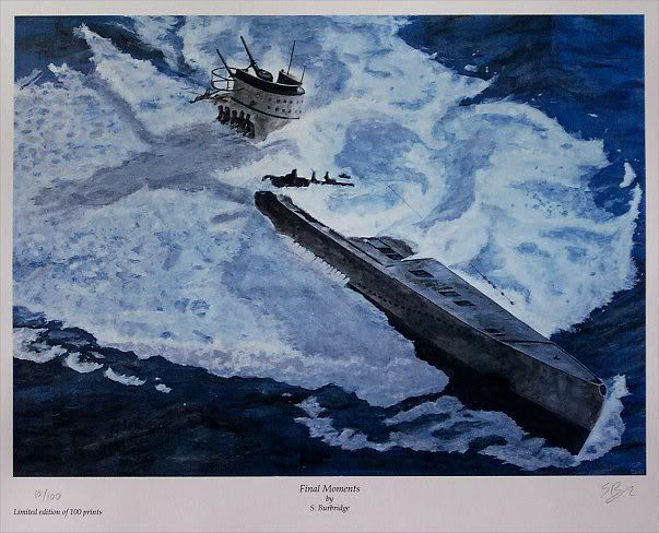
Image credit: S. Burbridge, “Final Moments”, subart.net
In the post war era, and throughout the Cold War, as the hard lessons (and promising technologies) of WWII were developed and improved upon, the punch and counter-punch of ASW continued to develop at a fervent pace.
This included such rapid post war developments as the teardrop hull form (derived from the USS Albacore (AGSS-569) design, circa 1948), the emergence of nuclear powered propulsion (from Admiral Hyman G. Rickover’s USS Nautilus (SSN-571), circa 1951), and the arrival of the ballistic missile submarine in the mid 1950s.
The evident teardrop hull form of the USS Albacore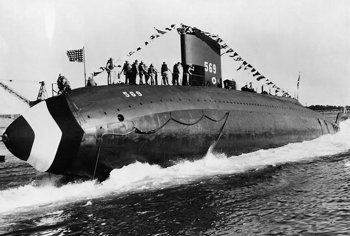
Image credit: US Navy.
Submarine warfare in the modern era has been much less exciting, or perhaps more accurately, much less outside the gaze of the public eye. The examples of successful engagements, both by submarines and against them, are fairly well publicised.
For example, the sinking of the Argentine cruiser General Belgrano by the British Royal Navy nuclear attack submarine HMS Conqueror during the 1982 Falklands war and, on the other side of the equation, the destruction of the Pakistani Navy submarine PNS Ghazi during the 1971 conflict with India.
Much less well known are the countless times during the Cold War when submarines have attempted to affect, directly or indirectly, the course of geo-political events by their very presence, without a shot ever having been fired.
For example, the deployment of HMS Dreadnought to the Falklands in November 1977 under the auspices of Operation Journeyman; or the report that a Dutch Walrus class sub was stationed off Kotor during the 1999 Kosovo conflict and tasked to engage any Yugoslavian submarines that might emerge to threaten NATO ships.
In modern times, submarines have been more notable for tasks that defy traditional undersea warfare, such as launching cruise missiles against distant shore targets, or delivering special operations forces ashore to conduct clandestine small unit operations.
Suffice to say, undersea warfare – both from the point of view of the submariner, and from that of those attempting to hunt him down – has been a complex, fluid, and militarily important affair. It remains so today. And, notably, the see-saw battle of how to find, hunt and destroy submarines – and on the other side, how submarines evade, hunt and attack their enemies – continues to push technological boundaries.
B. SONAR: THE MAINSTAY OF ANTI-SUBMARINE WARFARE (ASW)
Stealth is arguably the defining characteristic of the submarine. The foremost, and by far the most difficult task in the ASW cycle, therefore, is actually finding them.
The acronym ASW has sometimes been translated as “awfully slow warfare”, and this is probably a good description. A couple of anecdotal references serve to highlight this portrayal of ASW: Being in a submarine is like “being stuck in the boiler room of your high school for several weeks”; or, that the weather on a “sealed people tube” is always the same, “69 degrees and fluorescent”.
One can rest assured that it is an equally mind numbing exercise for the crew of the ships and aircraft that are scouring the ocean for a hint of an enemy submarine, the proverbial search for a “needle in a haystack”.
When ASW does get exciting, however, and perhaps more than a little nerve wracking, is when you finally do get that “contact”. So, the question naturally follows: How does one get (and ultimately prosecute) a contact?
1. Active Sonar
As we learned in Part 1 of this discussion, active sonar operates much like active radar, sending out a burst or pulse of sound energy (the “ping”) through the water, which then reflects off a target and returns as a reflection (or echo) to the sonar transducer.
A single transducer has little directional control over the ping, but by arranging or stacking multiple transducers in an array, and using special signal processing techniques, it is possible to use “beam forming” to send active sonar pings in specific directions.
The Sonar 2051 transducer array aboard Oberon class submarines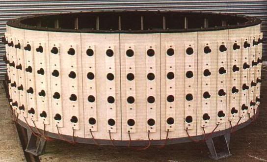
Image credit: web.ukonline.co.uk.
Generally speaking, the power of the transducer will dictate its maximum range. It also directly impacts signal frequency, since the longest ranges will be achieved with the lowest frequencies, and therefore only the largest transducer array will be able to produce the necessary long wavelengths.
All of this means that, in order to increase the transmitted power for a given array configuration, it is usually necessary to increase the size of the array. The necessity of a large sonar array obviously leads to physical limitations, especially when space aboard a warship or submarine is at a premium. Large arrays can add significant drag and require large power sources together with their supporting electrical and electronic equipment.
Hull mounted sonar arrays are typically cylindrical in shape, to give good coverage outward and downward, while those fitted to modern submarines are often spherical in shape, providing a much wider vertical field of view (useful in the subsurface environment, where you need coverage both above and below).
Active sonar arrays are generally mounted in the bow or keel, giving good coverage ahead of the ship, except in the area directly behind the array (the “baffles”; more on those later). Sound absorption materials are mounted directly behind the array, both to protect the occupants of the ship or submarine from the very loud sound energy (recall, up to 250 decibels!) and to prevent reflections back into the system. Streamlining and shielding around the array is done both to reduce drag and to reduce self-noise (including flow noise created by the passage of water around the array).
Modern surface ships and submarines are also likely to have a “suite” of active and passive sonars (a collection of bow, hull, flank, and/or towed systems) rather than relying on a single system.
Sonar suite on the Type 212 submarine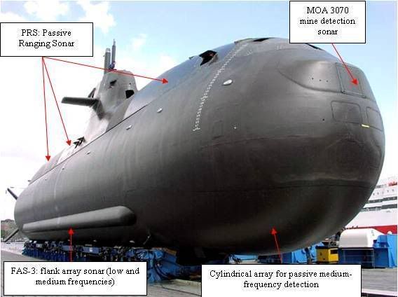
Image credit: Gerwalk, subpirates.com
As we discussed in Part 1, surface ships or submarines performing ASW will only rarely employ their active sonar, as it may be heard at over twice the distance (and given the proper acoustic conditions, much further) it can effectively return an echo. Banging away with active sonar in the blue water ocean environment typically serves only as a beacon for lurking enemies or, worse, invites a spread of torpedoes or cruise missiles in your general direction.
There are circumstances, however, where active sonar is useful or even preferable. (Always keeping in mind the drawbacks already mentioned, of course). For example, in shallow water, where your towed array is unavailable (due to the risk of it hanging up on the bottom) or where the topography prevents good acoustic conditions (e.g. no CZ formation).
Active sonar may also be your only useful choice when dealing with diesel-electric submarines, since these are extremely quiet when running on their batteries. Here’s an (alarming) analogy to get an idea of just how difficult (with thanks to Scott Gainer): Try to locate a refrigerator by listening for it from outside the house. 😮
2. Passive Sonar
The preferable approach for detecting enemy submarines has historically been the use of passive sonar. It is the instrument of choice for ASW, and as stated, active sonar is most often relegated to the attack phase or special circumstances.
As already discussed, passive sonar involves an array of dedicated hydrophones, or the receiver portion of an active sonar array, being used to “listen” for the acoustic signals generated by a target. As with active transducers, hydrophones can be arranged in an array to improve beamwidth and directivity.
A dedicated passive hydrophone array is much lighter and considerably less complex than an active transducer array, generally because it does not have the same high power requirements. Conformal arrays, placed alongside the length of the ship or submarine (often the latter), take advantage of this reduced weight and complexity.
As mentioned in Part 1 of this discussion, a ship or submarine’s self-noise, both narrowband and broadband in combination, forms its “acoustic signature”. This signature can be exploited by an enemy’s passive sonar to identify the target. For example, the broadband noise from a target’s propellers (generally of low frequency, less than 1000 Hz) can be detected and demodulated to measure the shaft or propeller blade rate (blade rate tonals) – a useful identifier. (Narrowband noise is typically plotted and shown on the famous “waterfall display”).
3. Variable Depth Sonar (VDS)
To improve the ability to hunt for submarines that might be hiding in shadow zones or below the thermocline (the “layer”), the Variable Depth Sonar (VDS) was developed in the 1950s. A VDS employs a streamlined body (the “fish”) which contains the transducer and is towed behind the ship. In conjunction with the speed of the ship and the length of the tow cable, and by employing control vanes and depth sensors, the fish can be deployed at depth.
The principal advantages of VDS, of course, are the ability to move the transducer away from the ship’s self-noise, penetrate the layer, and provide 360 degree coverage by placing the transducer behind and below the baffles.
VDS does have its limitations, however. Early models (such as the SQS-9) were streamed over the side, a rather cumbersome method, though in later practise the fish was streamed from the fantail via a hoist or winch system. The system does restrict ship maneuverability while in operation, and its bulky equipment is difficult to handle during inclement weather.
Thales TSM 2640 Salmon VDS aboard Royal Danish Navy frigate Thetis (F357)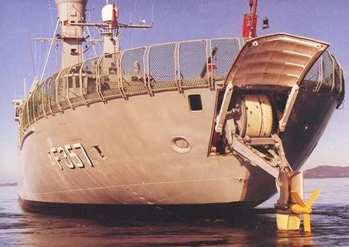
Image credit: Naval Technology, SPG Media Limited.
In recent years, the VDS has been supplanted by the linear towed array for ASW work, while VDS systems have become more specialised tools in the field of mine countermeasures (MCM). In this role they are often equipped with high frequency side scan sonars which are short ranged but provide excellent resolution, sufficiently high in most cases to perform imaging of the bottom and object classification.
4. Towed Arrays
During the Cold War, when the North Atlantic was the main hunting ground of both NATO and Warsaw Pact submarine forces, the low frequency passive towed array sonar emerged as the prime ASW sensor for surface ships. Exploiting advances in signal processing, and taking advantage of the excellent acoustic propagation characteristics in the deep sound channel (DSC), towed arrays were capable of detecting and holding contacts at ranges at dozens of miles.
Unlike a VDS, in which the sonar array is encased in a streamlined body or “fish” at the end of a relatively short tow cable, the towed array or “streamer” comprises a hose or sheath of an elastomeric material (such as rubber) between 2 and 4 inches in diameter and containing numerous transducers (typically of ceramic piezo-electric design) or receivers arranged in a linear fashion. The array can be thousands of feet (even miles) in length.
The towed array’s sheath is filled with an acoustically transmitting material (typically a fluid) that provides structural integrity, dissipates internal heat, and provides some isolation from flow noise. Since the array’s diameter has a direct correlation with flow noise, it is desirable to reduce the diameter of the array to as small as possible. This is difficult from an engineering point of view, but even so, modern “thin line” towed arrays have been able to achieve a minimum diameter of about one inch.
In addition to the engineering and design obstacles, towed arrays have their own characteristic problems: these include boundary layer noise; internal self-noise caused by waves propagating between transducers inside the array; or external self-noise or “cable strumming” caused by towing the cable through the water. The cable may vibrate, that vibration is passed into the array, and is picked up by the transducers.
A fundamental problem with towed arrays is that the position of the hydrophones or “nodal points” within the array is inherently unstable. Because of ocean currents, their position in the array, the speed of the host platform, or other factors, their relative positions are changing continuously. Because of the negative effect this can have on acoustic properties, it is important to monitor the relative positions of the nodal points of the array at all times. One common method is to use multiple “birds” clipped onto the tow lines, each comprising a transducer used to calculate the range between nodal points. The results are used to determine the shape of the array, which in turn is critically important to its performance.
Towed array
Image credit: Federation of American Scientists.
Surface Ship Towed Arrays
Notably, towed array systems have offered the surface ship, for the first time, the possibility of parity with the submarine in passive sonar capability. The long range detections made possible by towed arrays are of limited value to surface ships, however, without some means of localizing and prosecuting an enemy submarine contact. And, of course, this is the function performed by aircraft acting in conjunction with the surface ship.
From an ASW point of view, the US Navy surface fleet evolved slowly from a sensor/weapon suite based on the SQS-26 hull mounted active/passive sonar set of the 1960s, the RUR-5 ASROC (Anti-Submarine Rocket) stand-off weapon, and the SH-2 Seasprite LAMPS I (Light Airborne Multi-Purpose System) helicopter.
By the mid 1980s, it had become a system based largely on variants of the SQS-53 hull mounted sonar first introduced in 1972, the SQR-19 TACTAS (Tactical Towed Array) passive towed array, and the longer range SH-60B Seahawk LAMPS III helicopter. (There never was a LAMPS II system).
Along the way, during the period of this evolution, the US Navy conducted:
(1) Its first experiments and deployment with the ITASS (Interim Towed Array Surveillance System) towed from VDS fish on the Dealey class destroyer escort USS Van Voorhis (DE-1028) in 1970;
(2) Its first experiments and deployment with an interim tactical towed array design (the SQR-18) on the Knox class frigate USS Moinester (FF 1097). The SQR-18 was a passive towed array some 800 feet long streamed from the SQS-35 IVDS (Independent Variable Depth Sonar) body on a tow cable nearly 5,600 feet long. (The SQS-35 was evolved from the EDO Model 983, a 13 kHz VDS).
(3) Its first experiments and deployment of a higher speed tactical array (the SQR-19) on the Spruance class destroyer USS Moosbrugger (DD 980) in the early 1980s.
The most recent, new generation towed arrays, such as the British Sonar 2087 and the US SQR-20 Multi-Function Towed Array (MFTA), employ both active and passive arrays, exploit the range advantages of the low frequency range, and are more tolerant of high speeds.
Submarine Towed Arrays
Submarines can deploy “fat line” towed arrays using a process known as flushing, wherein water is pumped into the tube to exert pressure upon and hence deploy the array. The US Navy’s TB-16 is an example of a fat line towed array, which consists of an acoustic detector array weighing some 1,400 lb, measures about 3.5 inches in diameter, and 240 feet long. The TB-16 array is towed at the end of a cable some 2,400 feet in length.
Alternatively, submarines may deploy “thin line” towed arrays using mechanical handling systems. A thin line array comprises an outer sheath or hose that contains the hydrophones and supporting wiring and electronics. When the array is deployed or retrieved, it is fed through a guide by a handling system. The US Navy’s TB-23 is an example of a thin line towed array.
Winch system for the Type 212 submarine’s TAS-3 towed array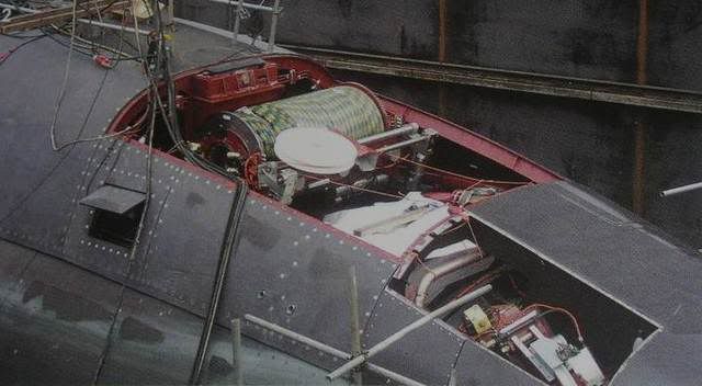
Image credit: Gerwalk, subpirates.com
Advances gained from commercial off the shelf (COTS) computer processing (such as that made available through the Advanced Rapid COTS Insertion, or ARCI, program) has substantially reduced cost while significantly improving processing power, which in turn permits the use of powerful new algorithms for better towed array detection ranges. The US Navy’s TB-29 thin line towed array, for example, is a version of the legacy TB-29 array utilising commercial off the shelf (COTS) telemetry.
Towed array technology has advanced rapidly with longer, multiple line systems that provide increasing number flexibility for submarine based ASW. Many existing Navy tow cable systems have single coaxial conductors, 1-2 kilometers in length, within which power, uplink data, and downlink data are multiplexed. These systems typically run at uplink data rates of less than 12 Mbit/sec due to the bandwidth limitations of a long coaxial cable.
Operational beam formers for towed arrays have traditionally assumed the array geometry to be straight and horizontal aft of the host platform, but in reality there is always some deformation in this geometry. “Chain link” and “stiff stick” models have been used to estimate towed array position and heading, but the newer arrays (such as the TB-29) are equipped with their own sensors to accurately determine the position of the array and its heading. This is more accurate than either of the previous methods, and will be used to optimise TMA solutions.
5. Dipping Sonars
Dipping or dunking sonars are a variant of the VDS concept. While principally fitted aboard helicopters, they can also be found aboard some small patrol craft and surface ships (such as the MGK-345 Bronza (NATO Rat Tail) dipping sonar found aboard Project 1241.2 (NATO Pauk) class corvettes).
While operating in the hover, a helicopter can use a winch and cable to lower a sonar transducer into the water and to the desired depth. Again, self-noise is minimal because the array is isolated from both the noise and vibration of the power source and the helicopter.
AQS-13 dipping sonar deployed from a Sea King helicopter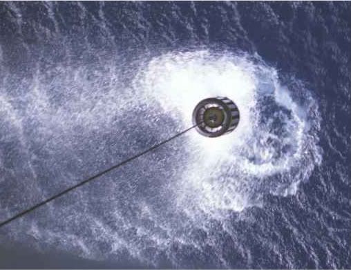
Image credit: http://www.solarnavigator.net
A helicopter dipping sonar typically consists of a “wet end” or transducer; a cable (at least 1,000 feet in length) and reel/winch assembly; and a “dry end”, consisting of the power supply and sonar processing systems.
There are, of course, no baffles or blind spots with a dipping sonar. It has full 360 degree capability, and for the size of the transducer, most are quite capable, with source levels exceeding 200 decibels (dB) and an effective range of several thousand yards. Newer systems also have a sonobuoy interface, allowing them to process the returns from three or more sonobuoys, and the ability to communicate with friendly submarines via underwater telephone.
Power was supplied to the transducer via a lead-acid battery in most older systems, and recharged between transmission cycles, but newer dipping sonars are powered directly by the helicopter rather than by a battery.
Helicopter dipping sonars have also joined the drive to enhance capabilities in the littorals, both in terms of locating ultra quiet diesel subs and in the mine countermeasures role. Examples of the latter include the AQS-14 and AQS-20 systems.
The new AQS-22 FLASH (Folding Low Frequency Active Sonar for Helicopters) system is being fitted to the new MH-60R Seahawk (as well as other types), and is claimed to provide submarine detection, tracking, localization and classification; acoustic interception; underwater communications; and environmental data acquisition, both in blue water and littoral zones. The AQS-22 transducer/receiver weighs only 100 lb and has a cable length of over 2,500 feet.
6. Jezebel, Julie, and Company: Sonobuoys
Sonobuoys are essentially expendable sonar devices typically deployed by aircraft, though they may also be hand deployed over the side of a ship. In fact, the first sonobuoys of early WWII were an expendable sensor towed behind convoy escorts and used to detect German U-boats attempting to approach from the rear. Their usefulness as an aircraft delivered sensor, however, was not fully appreciated until late in the war, by which time the US Navy finally ordered some 150,000 examples (mostly the CRT-1 type).
Sonobuoy development languished somewhat immediately after WWII, that is, until the quick pace of Soviet submarine development became an increasing concern and the SOSUS project began in earnest (more on SOSUS later).
In 1951, Project Jezebel combined LOFAR (Low Frequency Analysis and Recording) equipment with fixed hydrophone arrays (such as SOSUS), and aircraft became the means of rapidly prosecuting the SOSUS detections. Whereas SOSUS provided only the initial detection and a general area of probability, sonobuoys could be used for tactical level search and localization. Passive sonobuoys thus became known as Jezebel buoys.
Whether sonobuoys are parachute delivered from the air or dropped over the side of a ship, the launching platform must be equipped with the electronic equipment needed to receive and process the data being gathered and returned by the sonobuoy (typically via VHF transmitter).
The sonobuoy’s own battery (often silver chloride) power is activated by contact with seawater (though some types are now switching to lithium), and a mechanism for inflating a flotation device is activated, such that the transducer or receiver is suspended below the surface to a certain specified depth while the buoy (and antenna) remain floating.
Sonobuoys are classified by their size (A, B, C, etc.) and their type (active or passive, or measurement). Most US manufactured sonobuoys are A size, measuring about 4 7/8 inches in diameter and 36 inches in length. (An A/2 size buoy is a half size A type buoy).
A sonobuoy being dropped from a P-3 Orion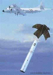
mage credit: National Oceanic and Atmospheric Administration (NOAA).
CZ do not form perfect concentric cylinders, of course, but rather a series of curved 3-D shapes, so it is quite possible that a submarine within CZ range but below the CZ path could remain undetected. The same is true for the areas between the annuli, where shadow zones will develop.
Both active sonar and passive sonar may make use of CZ. This is especially true of low frequency sound, the kind generated by a high powered active sonar such as that found aboard the American Spruance (DD-963) class and the Soviet (Russian) Udaloy (Project 1155) class ASW destroyers.
In the same way that radar warning receivers (RWRs) and electronic surveillance measures (ESM) gear can detect actively emitting radars well beyond their own effective range, actively emitting sonar can also be detected well beyond the range at which it can effectively receive an echo. As a rough rule of thumb, active sonar can be heard at three times the distance at which it can detect targets.
5. Direct Path and Bottom Bounce
Sounds in the ocean are rarely confined to following a single path, and each of those potential paths must be considered when using acoustic devices to try and detect or locate ocean objects. In addition to the CZ phenomenon, sound may travel by direct path or bottom bounce.
Direct Path
The direct path is, just like the term suggests, the simplest acoustic propagation path. It occurs in the surface layer, and acts much like radar, being essentially a straight line path between the sonar source and the target, with no reflection and only a single change in direction due to refraction. It is the principle upon which fathometers are based.
The maximum achievable range obtained by exploiting the direct path is tied directly to the point at which the surface duct limiting ray is reflected from the surface. For most hull mounted medium frequency sonars, maximum direct path range is typically less than 10 nautical miles (nm), and most often, much shorter than that. (Range is of course largely dependent upon the power and frequency of the sonar in question).
Bottom Bounce
Bottom bounce is an acoustic propagation path that involves reflecting sound off the bottom, so that it “bounces” up to the surface, and then is reflected downward again. It is chiefly an effect of medium (MF) and high frequency (HF) sonars, since low frequency sound tends to be absorbed into the bottom.
Bottom bounce normally occurs in areas where the bottom is fairly smooth and the water depth is slightly greater than critical depth (see our earlier discussion on that term), typically in depths greater than 2,000 meters but less than 5,000 meters. It is useful in shallow seas, such as the Mediterranean, or along the deeper portions of the Continental Shelf.
The angles at which the sound enter the water during bottom bounce are generally too steep to produce the sort of refraction that results in CZ (that is, provided the depth is less than 5,000 m), and are typically between 15 and 45 degrees from the horizontal. Maximum effective range for the bottom bounce technique is less than 20 nautical miles.
The chief advantage of the bottom bounce technique is that it can fill the gap between relatively short direct path range and long distance CZ detections, particularly where conditions limit CZ propagation. It isn’t as popular in the modern era, largely due to higher than expected absorption rates across much of the ocean floor.
Bottom bounce
Image credit: ES310, Introduction to Naval Weapons Engineering.
C. TACTICAL OCEANOGRAPHY IN ANTI-SUBMARINE WARFARE
What does all of this mean in anti-submarine warfare (ASW)?
Simply put, it means that ocean conditions have a huge influence on how ASW sensors and weapons behave. Because of this influence, it is critically important to be aware of the conditions in which your submarine (or surface ship) is operating.
1. Ocean Depth and Topography
As discussed, water depth, bottom contour, and bottom composition will affect sound propagation, and in turn, sonar performance.
If the sound source is deep and the conditions are right, sound propagation may occur in what is referred to as the “deep sound channel” or DSC (previously called the SOFAR channel, or Sound Fixing And Ranging Channel). Sound is “trapped” in the DSC, with no losses at its boundaries, in turn providing extremely low loss to the receiver. (This is similar in principle to the transmission of light in a fiber optic cable). Low frequency sounds can travel for literally thousands of miles in the DSC.
The famous US Navy SOSUS (Sound Surveillance System) – the chain of bottom laid hydrophones devices strung across the north Atlantic – exploited the deep sound channel phenomenon to listen for Soviet submarines.
The DSC tends to occur deeper near the Equator, and shallower at the Poles. You can even achieve similar propagation in the surface duct under ideal conditions, but there are always some reflection loss at the surface.
The deep sound channel, here at around 750 meters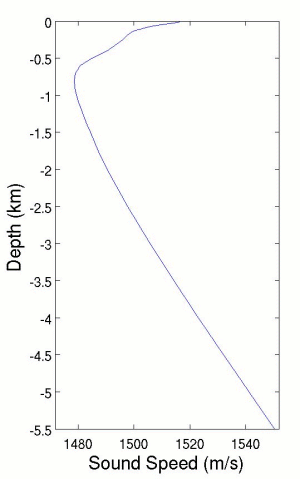
Image credit: World Ocean Atlas, US National Oceanographic Data Center.
Sound propagation is also affected by absorption in the water itself as well as at the surface and bottom. Sonars tend to perform best where the ocean bottom is hard and flat, and worst where it is muddy (or rocky, in which case, you get more scattering than absorption). This absorption is frequency dependent, as we discussed earlier, with highest frequency sounds being absorbed first, and lowest frequency sounds last. This is why sonars required to operate over long ranges tend to utilise low frequencies to minimise absorption effects.
In shallow water, sound propagation can suffer considerable loss. Certain sonars, for example, such as low frequency types, tend to perform poorly in shallow waters due to reverberation (scattering) and the harmonic noise produced by wave action.
Since underwater topography also influences sound propagation, submariners try to remain aware of features such as ocean ridges, sea mounts, guyotes (which are flat topped features that look like underwater mesas), and islands. The composition of the ocean bottom can likewise influence the performance of bottom bounce sonar or affect the placement of mines. Another obvious, and ominous, reason to remain aware of undersea topography is the hazard they can pose to subsurface navigation. Witness what happened to the USS San Francisco (SSN-711) in April 2005: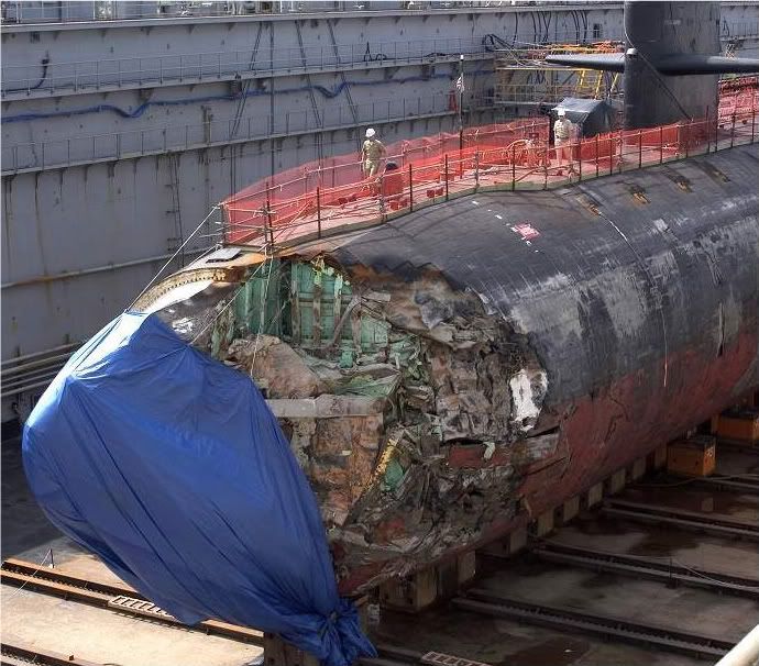
Photo credit: US Navy.
2. Ocean Temperature and Salinity
Another consideration is the freshwater outflow from rivers and the outflow from marginal seas, which can significantly affect sound propagation characteristics.
This is because, as we learned earlier in this discussion, both temperature and salinity will affect the speed of sound underwater. In turn, the behavior or performance of active and passive sonar is affected.
The temperature and salinity levels of the ocean vary widely between geographical regions. In the Arctic, low water temperatures can make for nearly uniform conditions from the surface to the ocean floor, which ordinarily might make for consistent sonar performance. However, the presence of ice also means obstacles to sound propagation (increased potential for scattering and reverberation) and high amounts of ambient noise (due to the constant grinding of the ice pack).
Varying salinity levels can also affect sonar performance. For example, the Mediterranean salinity “tongue”, the name given to the warm outflow of water passing through the Strait of Gibraltar into the Atlantic, forms a mass of water that stretches nearly all the way to Bermuda and possesses acoustical properties that are distinct from other ocean regions.
Image credit: Dynamics of the Mediterranean Salinity Tongue, James C. Stephens and David P. Marshall, in Journal of Physical Oceanography, Vol 29, Issue 27, July 1999.
3. Ambient Noise
Even without ships and submarines present, the ocean is far from a quiet place. The ocean’s own background noise, or ambient noise, varies widely with source, location, and frequency. Turbulence and geologic or seismic activity (such as underwater volcanoes) are the primary contributors to low frequency ambient noise. Ports and harbors will have increased localized noise levels due to industrial activity and merchant traffic. Distant ship traffic is perhaps the dominant noise source in the range of medium frequencies. Surface noise, such as wind and wave action, or rainfall on the surface, is the primary source of high frequency ambient noise.
Biological activity in the ocean also contributes to ambient noise and can influence your sonar. (Look up the fascinating story of the snapping shrimp). Tropical waters year round, and temperate and polar waters in the summer time, are especially prone. Marine mammals, especially toothed whales and dolphins, naturally use a method of echo location (or biosonar) to communicate and find food. These sounds add to the cumulative background noise of the ocean. (There is considerable controversy, as well, surrounding the use of high powered military sonars in the world’s oceans and the negative effect it is believed to have on these same marine mammals).
The most obvious contribution to ambient noise is what is happening on the ocean’s surface due to weather. Higher winds drive bigger waves, and consequently cause a greater amount of noise. Consistent wind speed is measured by the Beaufort Wind Scale, ranging from 0 (calm, wind speed less than 1 knot) up to 12 (hurricane force, wind speed over 64 kt). There is a direct relationship, then, between the steady wind speed and the sea state (the height, period and character of the waves). The World Meteorological Organization (WMO) sea state codes set out a scale for assessing the condition of the ocean surface, ranging from 0 (calm, glassy seas) up to 9 (phenomenal waves, over 14 meters high).
The greater the size of those crashing waves, of course, the greater the ambient noise contribution. Weather tends to degrade sonar performance, as increasing sea states increase ambient noise in the surface duct. This can deafen hull mounted surface ship sonars, and likewise, mask the presence of surface ships from submarine sonars. (The frequency of the noise from sea state tends to be greater than 300 Hz).
4. Self-Noise
Self-noise is the noise that your own surface ship or submarine produces, and which may be detected by your own sonar (or, worse, by the enemy’s sonar system) and which contributes the overall degradation of sonar performance. Self-generated noise has therefore always been a problem for sonar platforms. Essentially, the faster a ship or submarine travels through the water, the more noise it creates and the less it hears. In both instances, it risks destruction by slower moving, stealthy opponents. The combination of a ship or submarine’s self-noise, both narrowband and broadband, form its “acoustic signature” and can be exploited by an enemy’s passive sonar to classify the vessel.
The noise from a ship or submarine’s machinery, propellers, and even the sound of the hull passing through the water (flow noise), all add to self-noise.
Ships and submarines have plenty of potentially noisy machinery, including their engines, reduction gears, generators, hydraulics, pumps and turbines. In addition to their own noise, machinery produces vibrations in the hull that are in turn passed into the surrounding water. Machinery noise is generally independent of speed, as it is masked at high speed by flow noise, and forms the major component of self-noise at low speed. Even electronics and electrical devices can produce noise (thermal noise) if inadequately shielded.
Flow noise is generated by the turbulence of water flowing over the hull, and is dependent upon speed, hull shape and, somewhat ironically, the placement of the sonar transducer.
Propeller noise (typically very low frequency) is dependent on rotation speed and the geometry of the propeller itself. In fact, cavitation noise is the loudest noise arising from normal ship operations. Cavitation occurs when partial vacuums or bubbles are formed by the motion of rapidly turning propellers (at high speeds), and when these bubbles collapse, they produce broadband noise that can be heard at a considerable distance (and also produce shock waves that can actually damage the propeller’s blades … remember the power of those snapping shrimp?).
Acoustic stealth can also be degraded by short, transient noises caused by such things as rudder movement, start up and stopping of machinery, a dropped wrench, or famously, the opening of the torpedo tube doors. Transient noises are very characteristic of submarines and can help classify them as such.
Unsurprisingly, navies have sought to reduce self-noise wherever possible in an effort to further enhance their own stealth. Vibration dampening, isolation, and shielding of noisy machinery and components, specially shaped or skewed propeller blade geometry, and pump jet propulsors, are examples of this effort. And, of course, crews exercise a serious noise discipline, particularly aboard submarines.
Considerable amounts of money and effort have been expended to find further ways to reduce the self-noise of submarines (and the surface ships that might hunt them), even since the days of WWII. One of the earliest efforts, one that continues today, was the addition of anechoic tiles or coatings to the hulls of submarines. The Kriegsmarine (German Navy) introduced the technology first in 1944, with a synthetic rubber coating for its U-boats called Alberich. Although the principle was (and is) sound, problems with the adhesive sometimes resulted in the coating coming off, flapping in the U-boat’s own wake and causing even more noise.
Modern anechoic tiles or coatings serve two purposes: to absorb active sonar, reducing the strength of the return and thereby reducing its effective range (which also reduces the acquisition range of active homing torpedoes); and to reduce self-noise, thereby reducing the effective range of an enemy’s passive sonar.
Clearly visible anechoic tiles on the bow of USS Key West (SSN 722)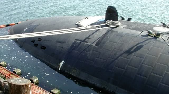
Photo credit: Rob Mackie, steelnavy.com, 7 October 2000.
A noise reduction system called “Prairie Masker” was developed by the US Navy for several classes of its warships (including the Spruance, Perry, Arleigh Burke, and Ticonderoga) to reduce or mask their self-noise. The Prairie system is fitted to the ship’s propellers, while Masker is fitted to the external hull in the vicinity of the propulsion plant. Compressed air is forced through machined perforations to create air bubbles that form a barrier around the propellers and hull, thereby shielding their radiated noise, and interfering with the ability of enemy passive sonar (particularly submarine sonar) to conduct analysis of the sound to classify or identify its source. It is reported that the acoustic signature of Prairie Masker sounds like rain to a passive sonar.
Prairie Masker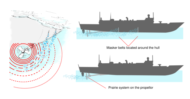
Image credit: Mariana Ruiz.
D. CONCLUSION
Hopefully this discussion has provided a decent foundation for an understanding of the anti-submarine warfare (ASW) environment, the “battlefield” in which submarines operate and their pursuers face off.
In Part 2 we’ll move to the tools of ASW – the sensors and the weapons.
Source references:
Jane’s Navy International, November/December 1995.
Naval Institute Guide to World Naval Weapons Systems, 1997-98.
Jane’s Information Group: August 1999; June 2003; September 2005.
Journal of Electronic Defense, March 2001.
Proceedings, June 2002.
National Defense, January 2003.
World of Defence, UDT, Issue No.2, 2004.
Navy Times, August 2005.
Harpoon 3 Sonar Model, AGSI, 2007.
Proceedings, June 2007.
ES310, Introduction to Naval Weapons Engineering.
Ocean Talk, Naval Meteorology and Oceanography Command.
uboataces.com
after searching i finally found this , hope you guy interested
ACTICS 101: ANTI-SUBMARINE WARFARE (ASW): PART 1 – THE FUNDAMENTALS
In Part 1 of this discussion, we’ll address the fundamentals of naval oceanography, i.e. the nature of the subsurface environment and how it impacts on anti-submarine warfare (ASW).
A. FEAR GOD, DREADNOUGHT, AND THE SUBMARINE!
The watchword of subsurface warfare, and by extension, anti-submarine warfare (ASW), is stealth. Submarines are absolutely dependent on stealth for both mission effectiveness and self-defense.
The introduction of submarines brought about a new and revolutionary dimension in naval warfare, one that was measurable in fathoms. Compared to the heavily armored ironclads, dreadnoughts, battleships, and battlecruisers that ruled the surface, directly confronting each other in hails of gunfire, a submerged submarine instantly became invisible, allowing it closely approach the most powerful surface ship. It could then deliver a torpedo, a weapon which could avoid the armor and strike below the waterline, where a ship was most vulnerable, thus allowing the smallest submarine to sink the largest ship.
This unique combination of stealth and offensive punch has therefore been the defining characteristic of the submarine from the very beginning.
British Admiral Sir John Fisher, the father of the the first big gun battleship, HMS Dreadnought, had the prescience to know that the submarine would seriously constrain surface ship operations, so much so that during WWI, the Grand Fleet did not operate in the southern part of the North Sea because of the threat posed by U-boats. Fisher had hoped to develop a blue water force projection capability that would combine the surface strike firepower of the battlecruiser with the submarine, making both the open ocean and the narrows untenable for the enemy. He envisioned that that the future of naval warfare lay in the ability to move quickly and strike at long range, as well as to go below the surface. Unfortunately for the Allies, Fisher’s vision proved to be ahead of its time.
The goal of modern ASW has remained unchanged from the time that the effectiveness of submarine warfare was first demonstrated during WWI. That goal is to deny an adversary submarine the ability to exercise its considerable influence on military objectives throughout an area of interest.
ASW no longer involves destroyers and corvettes racing around, pounding the ocean with active sonar and dumping seemingly endless numbers of depth charges on the heads of hapless and terrified submariners. (Though, admittedly, popping the movie Das Boot into the DVD player is still a favorite pastime).
Image credit: Das Boot, 1981, Columbia Pictures et al.
Rather, in the modern era, passive sonar is the instrument of choice (on both sides of the equation) when it comes to trying to detect and locate an enemy, and active sonar is usually relegated to the final attack and other special circumstances. Therefore, since passive sonar is so critically important, both surface ships and submarines take every effort to reduce their acoustic signatures.
Despite their stealth, submarines are inherently quite vulnerable, and they are easiest to detect when they poke their masts (or their hulls) through the surface. In an encounter between a surface ship and a submerged submarine, however, the advantage most definitely shifts to the submarine, as it tends to have a quieter acoustic signature.
This advantage diminishes significantly, however, when the surface ship can act in concert with other friendly assets, especially aircraft. In fact, aircraft are perhaps the most effective way of countering submarines.
More on that later, but firstly, let’s examine the environment in which submarines operate.
B. NAVAL OCEANOGRAPHY
1. The basics of SONAR
When the first sonar (sound navigation and ranging) systems were developed (the ASDIC system) between the world wars, it was believed that submarines would henceforth be stripped of their stealth. As was made obvious during the Battle of the Atlantic in World War II, this was hardly the case.
Sonar exploits underwater sound propagation to navigate, communicate, or as a means of acoustic location. There are two kinds of sonar: active and passive.
Active Sonar
Active sonar requires a transmitter to create a sound pulse (the famous “ping”) and a receiver, to “listen” for the reflection (the echo) of that sound pulse.
“Give me a ping, Vasili. One ping only, please.”
For snarf.
With active sonar, the source of the sound is the sonar system itself, the transducer (which converts electrical energy into acoustic energy). You also need a receiver to catch the signal (echo) reflected back from the target. That signal is degraded with increasing distance to the target in exponential fashion, so that four times the power of the active sonar produces only about twice the range.
A modern hull mounted active sonar can produce hundreds of thousands of watts of sound energy, reaching up to around 250 decibels (dB). Compare that to the sound level of a jet engine at 30 meters distance, which is just 150 dB!
Passive Sonar
With passive sonar, the sound source is the target itself. A transducer that can only receive acoustic energy is called a hydrophone.
Passive sources fall into two main categories: broadband and narrowband.
Broadband sources produce acoustic energy over a wide range of frequencies. When it comes to ships and submarines, typical broadband sources are noises that emanate from the propeller or shaft, flow noise, and some kinds of propulsion systems (e.g. steam boilers).
Narrowband sources, on the other hand, produce acoustic energy within a small band or class of frequencies. Typical ship and submarine sources are the various pieces of machinery found in every ship. For example, pumps, motors, electrical generation equipment and propulsion systems. When specifying narrowband sources, it is important to also specify the frequency at which it occurs.
Each type of sonar is dependent on a different characteristic of the sonar target that in turn influence sonar performance. For active sonar, that characteristic is the target’s sound reflection characteristics, or “target strength”. For passive sonar, the target’s own radiated noise is critical.
Frequency
Lower frequency (longer wavelength) sounds – generally in the 1-5 kHz range – tend to propagate the furthest distance, and require a large sonar dome to maintain gain (directionality). Medium frequency sonars fall generally into the 5-15 kHz band, and high frequency in the 20-30 kHz range.
High frequency (shorter wavelength) sonar can be broadly associated with short, direct path ranges in the surface layer (again, more to follow). Medium frequency sonars can be used to detect targets below the surface layer, and can sometimes exploit the bottom bounce technique. Low frequency sonars, meanwhile, have the potential to achieve convergence zone (CZ) detections. More to come on the terms direct path, surface layer, and bottom bounce.
It is also very important to note, however, that in recent years, the distinctions between frequency classifications and capabilities (as well as the boundaries of the frequencies being achieved) have blurred somewhat as technology has pushed the boundaries of what sonar can do. It is also important to realize that the ocean environment (including such variables as temperature, salinity, depth, and even geographic location) plays a huge role in affecting how sonar behaves, and notably, what it can and cannot do.
2. The Characteristics of Sound in the Ocean Environment
While light is highly absorbed by water, sound waves are not. Sound waves can thus be effectively used to probe the ocean’s depths, communicate underwater, and most importantly for the purposes of this discussion, locate submerged objects.
It is notable that although sound travels vastly farther through water than does light, it is lost in reverse order, i.e. highest frequency sounds are absorbed first, and lowest frequency sounds last. This frequency loss is also one reason why it can take quite awhile to determine the nature of, or develop, a sonar contact. It requires analysis of many sounds of many different frequencies, coming from different sources on the target, to determine its identity.
The speed that sound travels underwater varies from about 4,750 feet per second (fps) to about 5,150 fps. Its speed increases with:
1. Temperature, at a rate of about 4.3 fps per degree Fahrenheit.
2. Salinity, at a rate of about 4.3 fps per thousandth part increase in salinity.
3. Depth, at a rate of about 1 fps per 60 feet of depth.
The speed of sound underwater (in fps) can be determined as follows: 4388 + (11.25 × temperature (in degrees Fahrenheit)) + (0.0182 × depth (in feet)) + salinity (in parts per thousand)
(A special instrument, called a sound velocimeter, can be used to measure the sound velocity profile of a certain area of the ocean).
The average salinity of the world’s oceans is 35 parts per thousand (ppt), that is to say, the same as 35 grams of salt dissolved in each kilogram of water. Salinity in the oceans varies from about 32-37 ppt, except in the polar regions and near the shore (where fresh water from ice and the flow from rivers and streams act to dilute the salinity), where it may be less than 30 ppt.
Weather will also influence salinity, particularly where precipitation exceeds evaporation (such as in the rainy North Pacific) or where evaporation exceeds precipitation (such as in the Indian Ocean). An isolated body of water also tends to have higher salinity, such as in the Mediterranean, where excess evaporation works to increase salinity.
The polar seas (the Arctic and Antarctic) are the least saline (at 30-33 ppt), followed by the Indian Ocean (32-35 ppt), the Pacific (32-36 ppt), and lastly, the most saline ocean is the Atlantic (at 34-37 ppt).
Water pressure, which increases with depth, also has an effect on the propagation of sound. As stated, the speed of sound underwater increases with greater depth (i.e. increased pressure), which causes sound waves to bend (or refract) away from the area of higher sound speed. More on the effect of refraction in just a bit.
Let’s look more closely at one of the most significant factors affecting underwater acoustics: temperature.
3. The Thermocline or the Layer
The world’s oceans are stratified vertically with respect to temperature. Considered globally, seawater has a relatively large temperature range that depends upon location and time of year. Water temperature in the open ocean varies from a low of 28.4 degrees Fahrenheit (-2 degrees Celsius) to about 86 degrees F (30 degrees C), and can reach nearly 100 degrees F (37.8 degrees C) in shallow coastal waters around the Equator.
The thermal structure of the ocean is divided into three zones:
First is the surface layer or the mixed zone, where temperatures are almost uniform with depth. This is where waters are mixed together by wave action, solar driven circulation cells, tides, and so on. The depth of the surface layer varies with location and season. During winter months, it becomes more defined at all latitudes, and may extend to depths of 1,000 feet or more in mid latitudes during stormy weather. In the polar regions, water can become thoroughly mixed in winter, so that it is very nearly the same temperature from the surface to the bottom. Under normal conditions, the daily temperature of the surface layer varies as little as 5 degrees.
The bottom of the surface layer or mixed zone is marked by the next zone, the thermocline, where the temperature begins to decrease rapidly with depth.
The third zone is the deep layer, where temperature decreases very slowly with depth.
Ocean layers
Image credit: ES310, Introduction to Naval Weapons Engineering.
Here we are most concerned with the characteristics (i.e. acoustic properties) of the thermocline.
There may be a number of seasonal thermoclines present, which vary in depth and numberin accordance with the season (being most numerous and extending to the the deepest depths during the summertime), and also, standing or permanent thermoclines which appear year around and usually occupy deeper waters than do the seasonal kind. (Thermoclines may be identified on a bathythermograph trace, abbreviated BT or XBT, which is a graph that measures temperature as a function of depth, with temperature normally on the horizontal axis, and depth on the vertical axis).
Distinct density boundaries appear at the various thermoclines that change the water’s acoustic properties. Within the surface layer, sound travels generally in straight lines (particularly at angles of less than 15 and more than 45 degrees relative to the horizontal from the source).
The “layer”
Image credit: ES310, Introduction to Naval Weapons Engineering.
However, sound tends to bend (i.e. refraction) as it passes through the thermoclines and tends to produce “shadow zones” above and below the angle of the sound. The boundaries of these shadow zones are referred to as limiting rays. As a result, much of the sound generated by surface sources is trapped in the mixed layer and can travel over substantial distances (sometimes called the “surface duct”).
Surface duct
Image credit: ES310, Introduction to Naval Weapons Engineering.
There are exceptions to this effect, a good example being in the Red Sea, where hot water seeping from thermal vents pool and accumulate at the bottom, and another example, in the polar seas, where extremely cold surface water is present. These produce reverse thermoclines with temperatures that increase with depth (rather than the usual behavior of decreasing with depth).
Unsurprisingly, submariners pay close attention to keeping an eye on where the thermoclines are located, and may pass across these boundaries periodically to listen for targets above and below the layer.
Submarines enjoy an additional beneficial effect, in that sound generated below the surface duct may often only be detected in the mixed layer within a 45 degree cone from the source. Surface vessels, and sonobouys dropped by aircraft, get around this obstacle by using variable depth sonars (VDS) and hydrophones. The detection gear is suspended below the layer to detect sounds under it.
4. Convergence Zones (CZ)
Convergence zones (CZ) are another effect caused by the refraction of underwater sound and are chiefly a result of changes in sound speed velocity as depth increases.
Sound waves traveling down into the depths (past the critical depth, where velocity matches that at the source) tends to bend or refract back toward the surface due to the increased pressure (and hence, increased sound velocity). Under the right conditions, the refraction creates parabolically arcing paths through the water, and when it reaches the surface, in a donut shaped area called an annulus, the sound is reflected back down again. Each focus at the surface is called a convergence zone (CZ). The process repeats itself until the sound waves have been attenuated or obstructed.
Convergence zone
mage: ES310, Introduction to Naval Weapons Engineering.
CZ require a minimum depth of about 400 meters in order to form, at which depth they have about a 50 percent chance of developing. The likelihood of CZ forming tends to increase with water depth, so a depth of 600 meters yields an 80 percent probability of CZ, with near certainty in even deeper water. In shallow water, the sound waves echo off the bottom rather than refract upwards. Notably, underwater topography, such as sea mounts and mid oceanic ridges, tend to disrupt CZ paths, as do ocean currents that have significant differences in temperature (e.g. the Gulf Stream).
CZ typically develop at about 30-33 nautical mile (nm) intervals, with the width of the annulus increasing with distance. The first CZ at 30-33 nm typically has a surface annulus some 3-5 nm wide; the second, at 60-66 nm, is about 6 nm wide; and the third, at 90-99 nm, has a width of about 9 nm. Fourth and fifth CZ are possible but rare. Notably, CZ ranges in the Mediterranean are reduced due to layers of warm water near the bottom.
Annulus
Image credit: ES310, Introduction to Naval Weapons Engineering.
SU-34 has no sonobouys, nor torpedoes – it is a 2-seat strike aircraft, not an ASW aircraft.
I know you are a Russian fanboy, but really!
And the ASROC has a small range from its launching ship – aircraft-dropped torpedoes can be carried hundreds of miles from where the aircraft took off from, if needed.
my bad, i mean the Su-32FN from what i know they have MAD and can carry small torpedo
Ok i understand that aircraft can carry torpedo very far but what iam questions is their abilities to detect submarine
radar and IR would be quite useless, MAD isn’t much better either, the only thing that would work is their
sonobouy which isn’t as good as ship sonar any way, so if a submarine can hide from ship sonar wouldn’t it be obvious that it can hide from aircraft sonobouy too?
F-15 was cheap in era when over 200 F-16 were produced in a year. and F-15 is 4 times the weight of Yak-130. There is not much difference in weight between T-129 and Mi-28NM.
.
empty Mi-28NM is 7000 kg while max loaded t129 is 4000 kg:confused::confused::confused:
you will be banned if you continue to promote your blog like this
honestly in the look department Russian and USA helicopter are so so so ugly compared to the European one ( apart from rah-66 and ka-52)
Witchcraft… witchcraft! Unpost immediately!
We all know that shaping the hull a little bit more and using a little bit more ram is like going from a bike to a Koenigsegg.
But jokes aside, i still havent seen anything apart from stealth that is new (and radar reduction has been going on since the 80’s). The biggest reflectors are gone now (aluminum hull + visible fan), composites are used pretty much on all surface areas (not sure if Rafale and Typhoon are using CFRP nowadays on the canards, at least Gripen is, meaning pretty much 100% carbon or glass fibre on all surface areas (apart from some areas with iridium oxide treatment and AFRP).
Even the shaping is good today (we see faceting clearly on Rafale just to mention a small detail). It has gone so far in the development that the biggest reflectors are the tiny missiles themselves! I think it is extrordinary that pretty much the only way to make the targets stealthier (by any noticeable margin) is to hide the missiles. And that can be done with a pod.
stealth have much more to do with shape than material, also if you want to put missiles pod on rafale and typhoon then i dont think they will be super agile any more, probably becoming something like F-18 e/f
and no you cant just shape the hull a little bit and put the little bit RAM on Rafale, eurofighter, gripen and hope their kinematic performance remain the same, the aircraft will be much heavier , slower, less agile, have less range
Do some research into what the “barrier coat” actually is. This conversation is over.
Ok my mistake but
one-quarter wavelength only applied to certain kind of RAM
Radar absorbent material (RAM) can be used in the original construction, or as an addition to highly reflective surfaces. There are at least three types of RAM: resonant, non-resonant magnetic and non-resonant large volume. Resonant but somewhat ‘lossy’ materials are applied to the reflecting surfaces of the target. The thickness of the material corresponds to one-quarter wavelength of the expected illuminating radar-wave (a Salisbury screen). The incident radar energy is reflected from the outside and inside surfaces of the RAM to create a destructive wave interference pattern. This results in the cancellation of the reflected energy. Deviation from the expected frequency will cause losses in radar absorption, so this type of RAM is only useful against radar with a single, common, and unchanging frequency. Non-resonant magnetic RAM uses ferrite particles suspended in epoxy or paint to reduce the reflectivity of the surface to incident radar waves. Because the non-resonant RAM dissipates incident radar energy over a larger surface area, it usually results in a trivial increase in surface temperature, thus reducing RCS without an increase in infrared signature. A major advantage of non-resonant RAM is that it can be effective over a wide range of frequencies, whereas resonant RAM is limited to a narrow range of design frequencies. Large volume RAM is usually resistive carbon loading added to fiberglass hexagonal cell aircraft structures or other non-conducting components. Fins of resistive materials can also be added. Thin resistive sheets spaced by foam or aerogel may be suitable for space craft.
Thin coatings made of only dielectrics and conductors have very limited absorbing bandwidth, so magnetic materials are used when weight and cost permit, either in resonant RAM or as non-resonant RAM.
That’s what the anti-stealth hype would lead you to believe.
The simple reality is that “stealth” aircraft have always been detectable by not only low-frequency radars, but also by higher-frequency radars such as those in fighters & missiles.
The key is that “stealth” shaping and materials DO substantially reduce for all frequencies the range at which that detection occurs (NOT prevent it), and at which tracking is possible. Yes, lower frequencies are less-affected than higher frequencies, but since the only weapons-guidance which the large (dictated by physics) low-frequency radars can do is with telemetry-guided missiles* (which are very subject to jamming) or beam-riding missiles (which are limited in maneuver, lest they lose lock on the guiding beam from the ground station), this is not much of a problem (especially since those large radars are nice targets for cruise missiles, etc).
* Due to the physics of what kind of radar can fit in a missile, missiles can only have high-frequency radar receivers or transmitters.
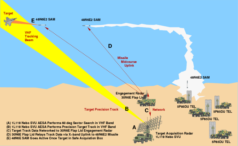
to be fair the Nebo SVU seem to be quite accurate , it can located aircraft in box of 5 km in height and 1.6 km in width (ok i know it from APA but still )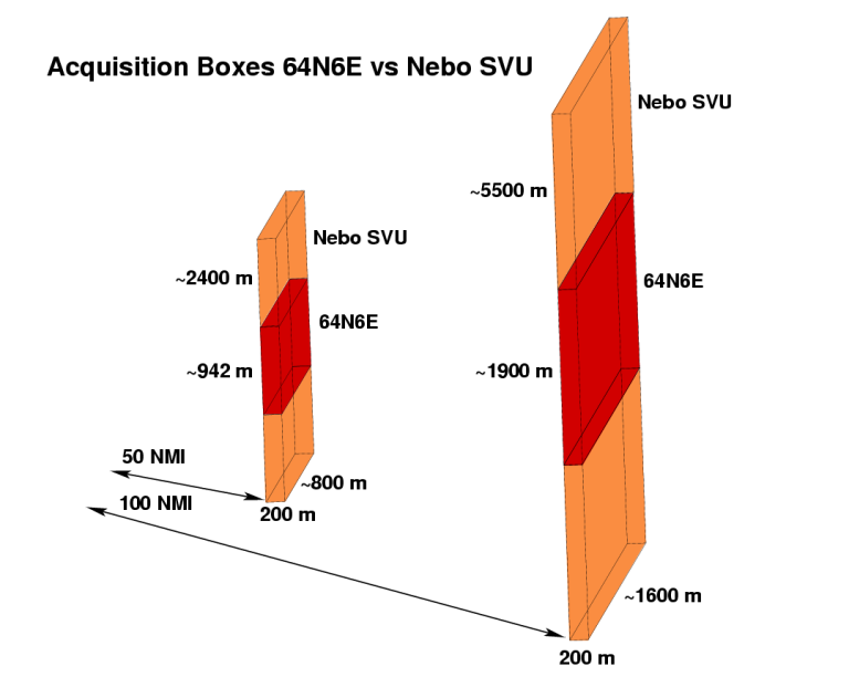
The radar’s cited angle measurement accuracies are 1.5° in elevation, 0.5° in azimuth, and range accuracy is 200 metres. This performance is almost identical to the S-band 64N6E Big Bird PESA used as a target acquisition component in the S-300PMU-1/2 Favorit / SA-20 Gargoyle and S-400 Triumf / SA-21 Growler SAM/ABM systems.
I think those numbers are cherry picked.
Its a while since I’ve been involved with CNF infused resins, but from what I remember:
– the weight difference is marginal (its only a small percentage of the overall resin weight that is changing).
– the material strength improves a reasonable amount (better transfer of load from resin to fibre and visa-versa.
– the material thermal expansion coefficients drop to a more isotropic behaviour pattern (CNF has low CTE and is not aligned to one axis)
– the crack propagation properties improve immensely (CNF bridging cracks and spreading load to fibre).
wasnt all these thing you listed are good thing ?
To have a CNT RAM effective @ the frequency range you’re jumping up and down about (and started this misguided thread on), the laminate would have to be 100mm thick!! Absorption of 10dB @ X- band does NOT mean absorption of 10dB at L-band for the same given thickness & composition.
you are talking about previous generation of RAM , it was addressed right in first post
old RAM
Low observable, or stealth, technology is utilized on aircrafts, ships, submarines, and missiles, for example, to make them less visible or observable to radar, infrared, sonar and other detection methods. Various radar absorbing materials (RAMs), which absorb electromagnetic frequencies, such as in the radar range, have been developed for such low observable applications. However, the RAMs presently employed have some drawbacks. For example, many RAMs are not an integral part of the surface of a low observable structure. Instead, the RAMs are applied as coatings or paints over the surface of the low observable structure making them heavier, and prone to wear, chipping, and failure. An example of such a RAM includes iron ball paint, which contains tiny spheres coated with carbonyl iron or ferrite. Moreover, these coatings require bonding to the surface of the structure because they are not an integrated part of the structure or surface.
Another example of a RAM is urethane foam impregnated with carbon. Such RAMs are used in very thick layers. Such RAMs are inherently non-structural in nature such that they add weight and volume to structures while providing no structural support. These types of foam RAMs are frequently cut into long pyramids. For low frequency damping, the distance from base to tip of the pyramid structure is often 24 inches, while high frequency panels can be as short as 3-4 inches.
Another RAM takes the form of doped polymer tiles bonded to the surface of the low observable structure. Such tiles which include neoprene doped with carbon black or iron particles, for example, are prone to separation, particularly in extreme operating environments such as extremely high or low temperatures, and/or high altitudes. Finally, numerous RAMs do not perform adequately in the long radar wavelength band, about 2 GHz.
It would be beneficial to develop alternative RAMs that address one or more of the aforementioned issues. The present invention satisfies this need and provides related advantages as well.
new RAM
The barrier coating can also be less than 10 nm, including 1 nm, 2 nm, 3nm, 4 nm, 5 nm, 6 nm, 7 nm, 8 nm, 9 nm, 10 nm, and any value in between.
Like I said, addition of exotic nanoparticles to enhance absorption will degrade mechanical strength. Also, what about thermal signature? The absorbed radar energy will be converted to heat.
not neccessary
also the heat is no where as high as normal friction caused by air when aircrafts fly at high speed , if you really worried about IRST you can always fly inside cloud
It’s a delicate balancing act pitted against ever more capable radars, algorithms & processing power.
lower RCS make jamming easier
as we learned earlier not only that lower RCS reduce burn through distance , jamming power required will decrease in the same rate as RCS reduction ,50% reduction in RCS = 50% less power required to overwhelm real radar reflection with noise ( you can work it out for yourself , 99.9% reduction in RCS= 99.9% less power required to achieve same level of effectiveness , and so on )
now let take example of 4 aircraft :
1) B-52 : RCS = 100 m2
2) Mig-31 : RCS = 10 m2
3) Mig-35 : RCS = 1 m2
4) F-35 : RCS = 0.001 m2
now compared them :
from B-52 to F-35 then RCS is reduced by 99.999% =>99.999% less power require
from Mig-31 to F-35 then RCS is reduced by 99.99%=>99.99% less power require
from Mig-35 to F-35 then RCS is reduced by 99.9% =>99.9% less power require
( if you not good at math then use this http://www.percentagecalculator.net/ the lowest row )so again a very powerful enemy radar : if F-35 need 5 kW jammer to shield it’s radar reflection with noise signals then Mig-35 will need a 5 MW jammer , Mig-31 will need 50 MW jammer , B-52 will required 500 MW jammer , you can argue that bigger aircraft can carry more powerful jammer but remember even the AEGIS only have power of 5 MW that why many countries start developing or buying LO asset because it much easier that way
jammer pod also improved in power
AN/ALQ-99 has a maximum power output of 27 kW http://mwrf.com/mixed-signal-semiconductors/gan-based-aesas-enable-us-navy-s-next-generation-jammer while NGJ capable of producing 60 kW-700 kW of power http://atgi.us/pdf/news/Aviation-Week-HiRAT.pdf , http://atgi.us/category/next-generation-jammer-ngj-program/#.VMdyJNLF-bN
there are also stand in jammer like MALD-J or AESA radar
Why do you find this development amusing?
Carbon nano tube material =much lighter weight ( 20-30% lighter) + effective again wide range of frequency
Low frequency radars have never been the silver bullet against stealth. Certainly they are capable of detecting fighter sized targets, but their large size means that they themselves are conspicuous and soft targets. Stealth is not foolproof, but neither are VHF radars.
i know but i have always thought that RAM have no use at low frequency
Notwithstanding the fact that CNT/fullerene RAM designed to be effective @ L & S band will be at the expense of other bandwidths (including X-band), these L & S- band CNT RAMs currently have an ‘upper limit’ where diminishing returns set in vis-a-vis LO design viability (and structural integrity where exotic nanoparticles are utilised).
It will be interesting to see how LRS-B, PAK-DA and upcoming heavy UCAVs address these future broadband stealth issues as radars attain ever greater power densities and advanced algorithms.
F.e, it would be interesting to know how the USN’s AMDR performs against LO targets as, evidently, future S & L band arrays and their associated systems will be a World apart from Nebo-M etc.
i think they stated clearly that the material is effective again frequency from 0.1 MHz to 60 Ghz which is included all VHF, Lband, Xband, Ka band


 Sign In